Exploring variable importance

While examining feature importance is most commonly thought of as something to do after building a machine learning model, it can and should also be done before performing any serious data analysis, as both a sanity check and a time saver.
Seeing which input features are the most predictive of the target feature can reveal potential problems with the dataset and/or the need to add more features to the dataset. Ultimately, narrowing down the entire feature space to a core set of variables that are the most predictive of the target variable is key to building successful data models.
Here you will find a collection of model-independent and dependent approaches for exploring the “informativeness” of variables in a dataset.
Unsupervised model-agnostic approaches
## Import libraries
library(FactoMineR)
library(factoextra)
## Loading required package: ggplot2## Welcome! Related Books: `Practical Guide To Cluster Analysis in R` at https://goo.gl/13EFCZlibrary(plyr)
library(dplyr)
library(arulesCBA)## Loading required package: Matrix## Loading required package: arules##
## Attaching package: 'arules'## The following object is masked from 'package:dplyr':
##
## recode## The following objects are masked from 'package:base':
##
## abbreviate, write## Loading required package: discretization## Loading required package: glmnet## Loaded glmnet 3.0## Discretize "Tenure" with respect to "Churn"/"No Churn"
df$Binned_Tenure <- discretizeDF.supervised(Churn ~ .,
df[, c('Tenure', 'Churn')],
method = 'mdlp')$Tenure
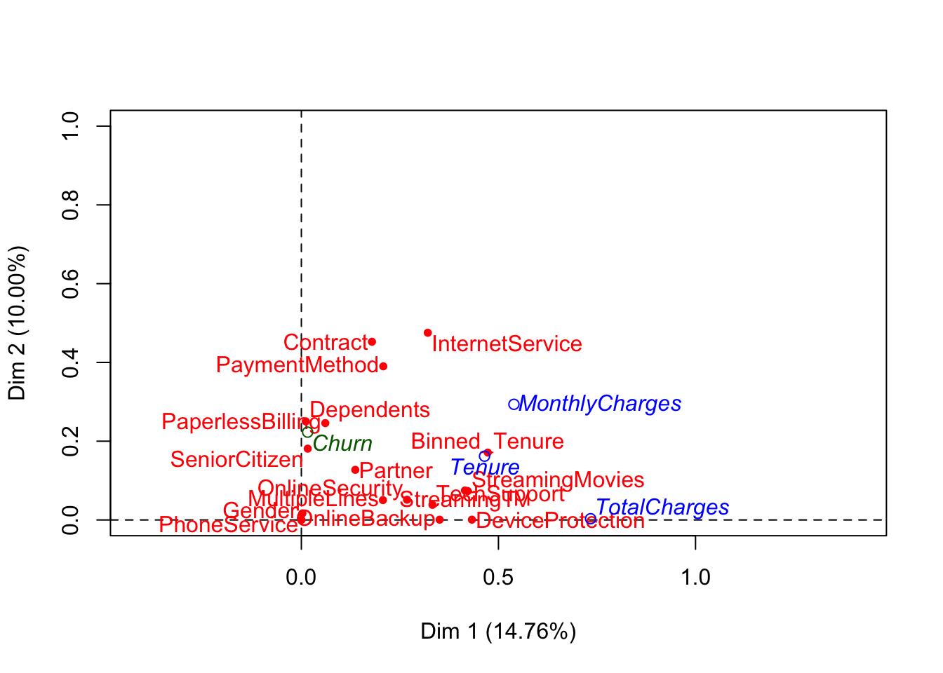
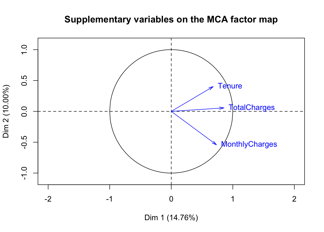
## MCA, with "Churn" set as the supplementary variable
res.mca <- MCA(df,
quanti.sup = c(5, 18, 19),
quali.sup = c(20))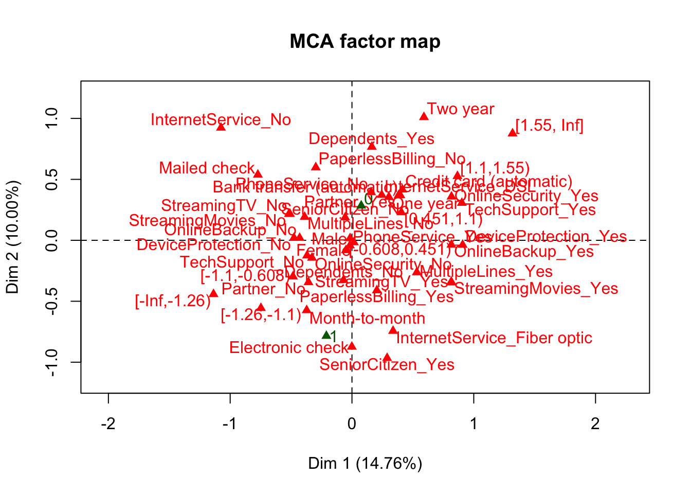
## Plot relationship between levels of categorical variables obtained from MCA
fviz_mca_var(res.mca, col.var = "cos2") 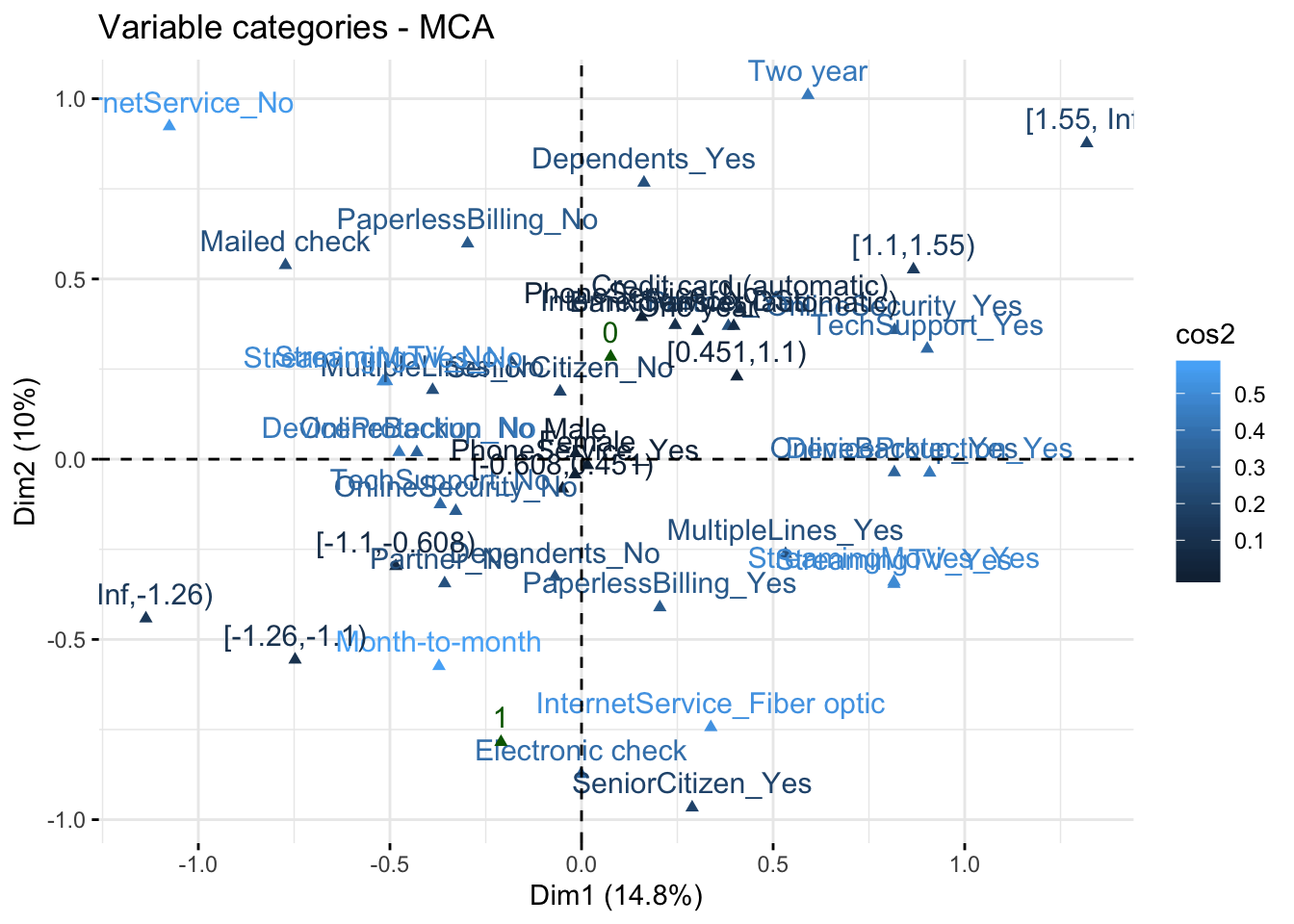
## Import libraries
library(ClustOfVar)
library(PCAmixdata)
library(dendextend)

## Split up continuous and categorical varibles
split <- splitmix(df)

X1 <- split$X.quanti

X2 <- split$X.quali

## Hierarchical clustering
tree <- hclustvar(X.quanti = X1, X.quali = X2)

## Evaluate the stability of each partition
x <- stability(tree, B=5) ## 5 bootstrap samples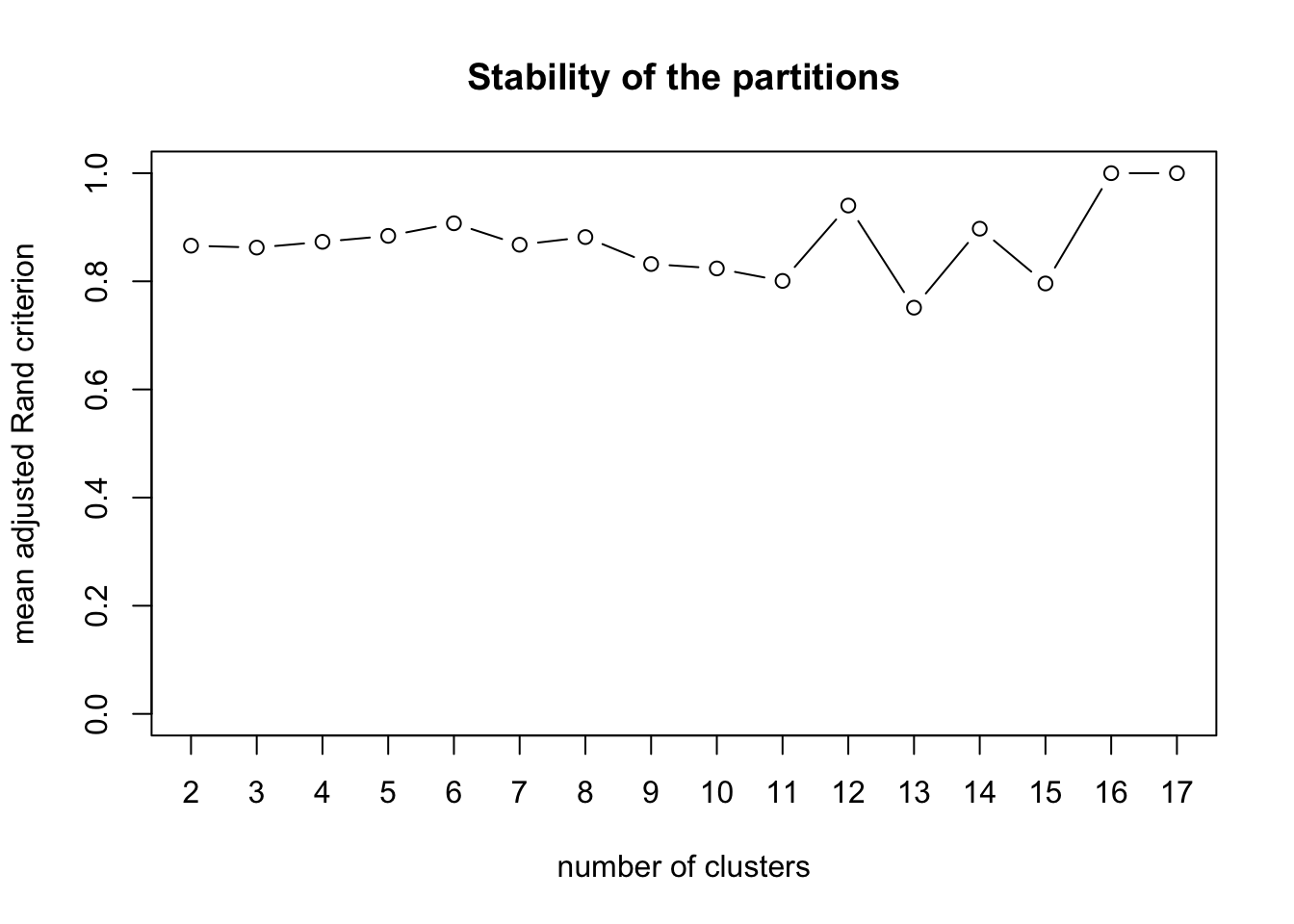
Plot the hierarchically clustered variables in a dendrogram:
par(mar = c(3, 4, 3, 8))

dend <- tree %>% as.dendrogram %>% hang.dendrogram

dend %>% color_branches(k=5) %>% color_labels(k=5) %>% plot(horiz=TRUE)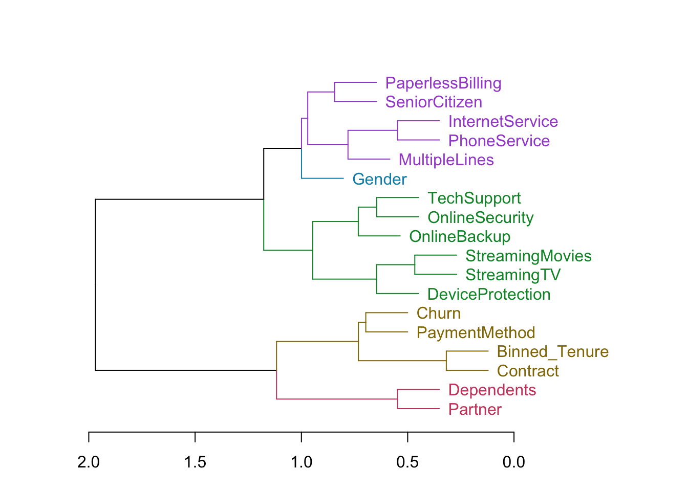
Supervised model-agnostic approaches
autoEDA
We have met the autoEDA package previously, as a tool for automated exploratory data analysis. In addition to making generating exploratory visualizations a breeze, it has a very cool predictivePower() function that calculates the “predictive power” of each input feature with respect to an outcome feature of your choice, which is quantified by correlation when the outcome feature is continuous and the Kolmogorov-Smirnov distance when it is categorical.
Note, the author of the package has warned that the estimation of feature predictive power is sensitive to how the data is prepared. Therefore, like all other tasks in data science, it is very advisable to put the same dataset through different analysis methods and see how the results match up.
Let’s give it a try for our outcome of interest, customer churn:
| Feature | PredictivePowerPercentage | PredictivePower |
|---|---|---|
| Contract | 46 | Medium |
| Tenure | 36 | Medium |
| Binned_Tenure | 36 | Medium |
| MonthlyCharges | 25 | Low |
| PaymentMethod | 24 | Low |
| TotalCharges | 22 | Low |
| InternetService | 21 | Low |
| PaperlessBilling | 21 | Low |
| OnlineSecurity | 18 | Low |
| Partner | 17 | Low |
| Dependents | 17 | Low |
| TechSupport | 17 | Low |
| SeniorCitizen | 13 | Low |
| OnlineBackup | 9 | Low |
| DeviceProtection | 7 | Low |
| StreamingTV | 7 | Low |
| StreamingMovies | 7 | Low |
| MultipleLines | 4 | Low |
| Gender | 1 | Low |
| PhoneService | 1 | Low |
ClustOfVar
## Import libraries
library(ClustOfVar)

## Calculate similarity between each variable and Churn
i <- 1

score_list = list()

for (c in colnames(within(df, rm("Churn")))){
  score_list[[i]] <- mixedVarSim(df[[c]], df$Churn)

  i <- i + 1
}

## Concatenate the two lists to a dataframe
score_df <- do.call(rbind,
                    Map(data.frame,
                        Var=as.list(colnames(within(df, rm("Churn")))),
                        Score=score_list))
## Import library
library(funModeling)
library(scorecard)
library(ggplot2)
library(ggpubr)

## Calulate variable importance
fM_imp <- var_rank_info(df, "Churn")

## Scorecard
sc_iv <- iv(df, y="Churn")

colnames(sc_iv) <- c('var', 'info_value')

## Combine the two
combine_df <- left_join(fM_imp, sc_iv, by = "var")

## Min-max scale result of each package, so they are comparable
normalize <- function(x) {
    return ((x - min(x)) / (max(x) - min(x)))
  }

dfNorm <- as.data.frame(lapply(combine_df[, 2:6], normalize))

x <- cbind(combine_df$var, dfNorm)

rownames(x) <- x[, 1]

x <- x[, 2:6]

colnames(x) <- c('Entropy', 'Mutual information', 'Information gain', 'Gain ratio', 'Information value')

## Make balloon plot
ggballoonplot(x, fill = "value", size.range = c(1, 7)) +
  scale_fill_viridis_c(option = "C")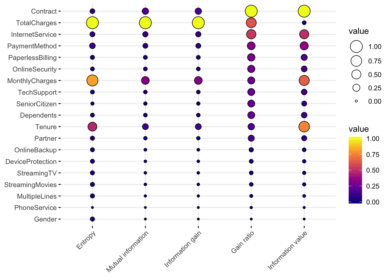
Model-dependent approaches
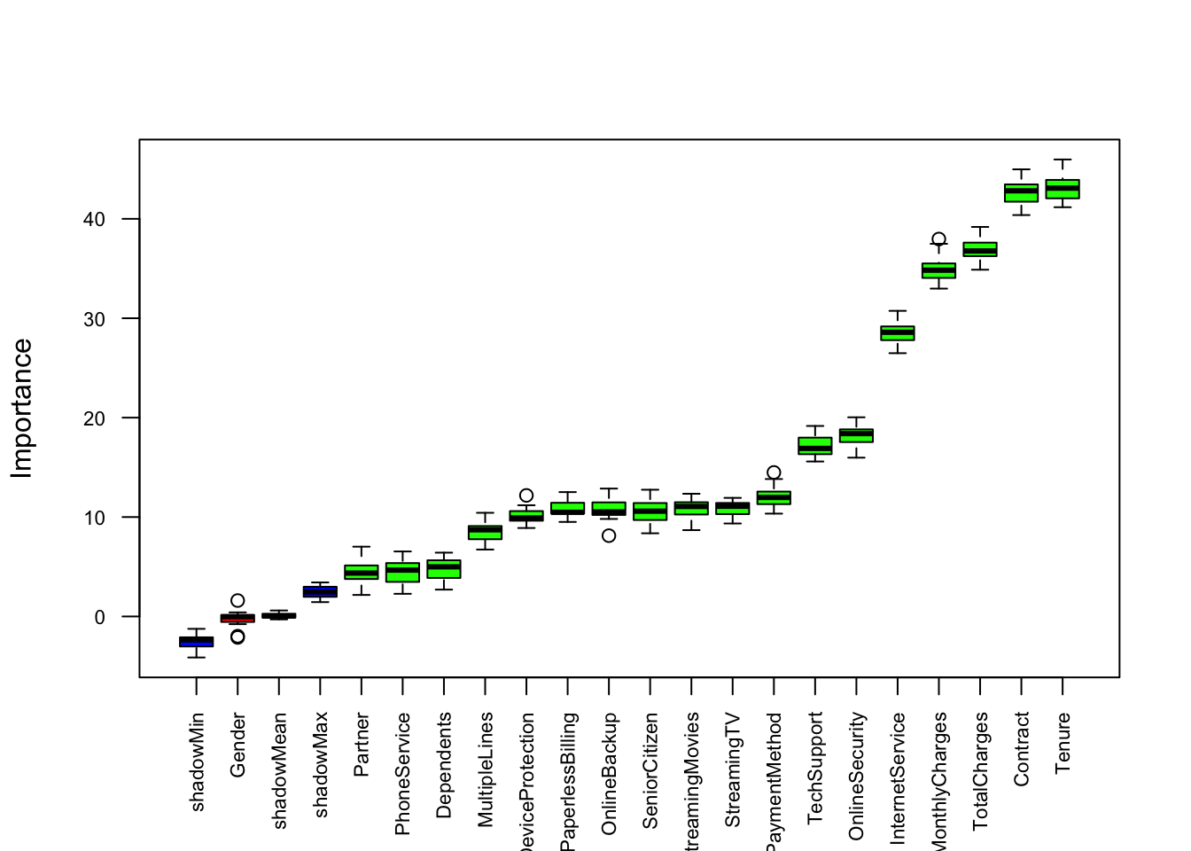
library(Boruta)## Loading required package: rangerset.seed(456)
boruta <- Boruta(Churn~., data=df, doTrace=0)
kable(boruta$ImpHistory) %>%
kable_styling(bootstrap_options = c("striped", "hover"))| Gender | SeniorCitizen | Partner | Dependents | Tenure | PhoneService | MultipleLines | InternetService | OnlineSecurity | OnlineBackup | DeviceProtection | TechSupport | StreamingTV | StreamingMovies | Contract | PaperlessBilling | PaymentMethod | MonthlyCharges | TotalCharges | shadowMax | shadowMean | shadowMin |
|---|---|---|---|---|---|---|---|---|---|---|---|---|---|---|---|---|---|---|---|---|---|
| 0.1356936 | 11.445128 | 3.809561 | 5.695892 | 42.16776 | 4.336411 | 7.258039 | 27.78640 | 18.79429 | 9.808921 | 12.178180 | 19.16411 | 9.876858 | 11.481957 | 43.20538 | 9.897038 | 11.35855 | 32.98180 | 35.92263 | 2.857294 | 0.0303948 | -2.304786 |
| -0.0402413 | 11.030769 | 5.085756 | 5.890952 | 42.84863 | 5.164849 | 6.732929 | 27.98407 | 18.39544 | 10.475808 | 9.020434 | 17.05949 | 11.626636 | 11.498145 | 41.86202 | 11.925629 | 12.39496 | 34.14153 | 34.88156 | 1.444568 | -0.2671151 | -4.125890 |
| -0.0259858 | 11.768550 | 3.711172 | 5.682888 | 44.08623 | 5.387057 | 6.856358 | 28.68633 | 17.75918 | 10.172381 | 11.187578 | 16.89430 | 11.897434 | 12.259004 | 43.87689 | 10.479638 | 12.37823 | 33.67295 | 36.55203 | 1.969644 | 0.2433086 | -2.357704 |
| -0.7747869 | 8.367250 | 7.020584 | 5.037047 | 41.64053 | 3.126726 | 8.108658 | 27.83533 | 17.75716 | 12.275353 | 10.758749 | 16.28029 | 9.353090 | 11.651878 | 40.96605 | 10.329537 | 10.34502 | 35.49940 | 36.76387 | 1.550604 | -0.1329682 | -3.765066 |
| 0.1044963 | 11.064880 | 5.179288 | 6.419857 | 43.29015 | 3.756288 | 7.482023 | 29.50315 | 16.62142 | 10.251592 | 11.022635 | 18.22732 | 11.157475 | 11.065602 | 41.58393 | 11.292338 | 11.24278 | 34.23869 | 36.86663 | 2.809089 | 0.2731351 | -2.160476 |
| -0.3291886 | 9.283133 | 4.043369 | 2.951300 | 41.16744 | 4.663319 | 9.117128 | 27.38804 | 18.66747 | 10.395198 | 10.441834 | 18.18472 | 11.087163 | 10.175477 | 43.50909 | 11.028153 | 10.77145 | 37.96813 | 36.70303 | 3.016841 | 0.6012491 | -2.023635 |
| 1.6016141 | 11.377006 | 4.493496 | 4.851501 | 43.50342 | 2.279622 | 9.388070 | 28.69641 | 17.23874 | 10.550455 | 9.812307 | 16.63531 | 10.587342 | 10.337582 | 42.80841 | 11.580611 | 13.82565 | 34.83401 | 37.33883 | 3.304929 | 0.1350296 | -3.644524 |
| -1.9833526 | 10.588582 | 4.053792 | 5.616524 | 41.39554 | 4.470852 | 8.973348 | 29.45276 | 17.14044 | 10.521982 | 9.969879 | 16.90613 | 11.149776 | 10.755274 | 41.07355 | 10.421386 | 10.91403 | 34.63494 | 37.19351 | 2.337012 | 0.3844707 | -3.390337 |
| 0.4089996 | 12.749351 | 3.160562 | 3.236891 | 43.08461 | 6.145945 | 8.509750 | 29.24886 | 15.97429 | 11.513107 | 9.912314 | 16.37133 | 10.269893 | 9.947096 | 43.14908 | 9.784528 | 11.46805 | 35.40394 | 36.22696 | 3.276767 | -0.1623191 | -2.623780 |
| 0.1548490 | 10.148420 | 3.728750 | 3.529062 | 43.04334 | 5.199150 | 7.917032 | 29.10187 | 20.03492 | 12.864714 | 9.585355 | 15.79663 | 9.366043 | 8.684432 | 41.25331 | 10.396281 | 12.49702 | 35.30919 | 38.25095 | 1.983142 | 0.2618099 | -1.245741 |
| -2.1084201 | 11.949892 | 3.260423 | 4.223116 | 43.44643 | 2.497987 | 10.259971 | 26.85989 | 17.33358 | 10.067193 | 9.808401 | 18.70230 | 10.716907 | 11.021818 | 40.37838 | 11.896557 | 12.62720 | 33.14540 | 38.71916 | 2.467228 | 0.0343937 | -2.946434 |
| -Inf | 9.180634 | 4.363038 | 5.395308 | 44.03111 | 5.356118 | 9.724825 | 30.74367 | 19.59800 | 11.438992 | 10.900286 | 17.79593 | 11.673326 | 9.061115 | 44.97793 | 12.510901 | 14.48827 | 35.34330 | 38.55780 | 2.775809 | 0.3261479 | -1.999441 |
| -Inf | 10.041568 | 2.165427 | 2.701832 | 44.31531 | 4.671867 | 8.599824 | 27.80714 | 18.32608 | 11.049520 | 8.939225 | 16.07197 | 11.232623 | 11.344527 | 43.93037 | 10.375393 | 12.26345 | 33.97118 | 36.26994 | 1.931157 | 0.0329752 | -2.035081 |
| -Inf | 11.639190 | 4.834238 | 5.836192 | 41.95306 | 6.020835 | 8.827196 | 27.85897 | 18.69084 | 11.592711 | 9.927759 | 18.61056 | 9.675507 | 11.234843 | 42.08601 | 12.363494 | 10.66494 | 34.71949 | 36.70988 | 3.382837 | -0.1050904 | -2.677616 |
| -Inf | 10.227206 | 5.926294 | 4.677897 | 41.91494 | 3.194645 | 8.727515 | 29.83875 | 19.78845 | 10.849001 | 9.831286 | 17.02572 | 11.333985 | 11.593612 | 42.81615 | 9.509118 | 11.54749 | 35.98680 | 36.21868 | 2.959059 | -0.2810412 | -2.290092 |
| -Inf | 10.086779 | 5.904646 | 4.829387 | 43.79991 | 3.202237 | 9.072997 | 27.47360 | 18.56422 | 8.126669 | 9.020453 | 17.75415 | 11.014845 | 10.548466 | 43.37546 | 10.841772 | 11.75929 | 35.52433 | 37.49800 | 3.422602 | 0.3428991 | -2.707708 |
| -Inf | 9.177680 | 4.573067 | 4.991486 | 45.96927 | 4.229134 | 8.713716 | 28.71831 | 17.83862 | 10.026637 | 10.069013 | 16.78743 | 11.501990 | 11.143915 | 42.74678 | 10.417723 | 12.73232 | 35.83626 | 37.71385 | 1.969737 | 0.1153363 | -3.085783 |
| -Inf | 9.365604 | 4.352948 | 3.166828 | 42.98059 | 5.488087 | 7.624188 | 26.48458 | 18.84666 | 12.576935 | 9.678820 | 15.74183 | 11.928859 | 12.342695 | 43.58864 | 10.227816 | 12.66173 | 37.48989 | 39.18548 | 2.166790 | 0.0480508 | -1.838376 |
| -Inf | 11.068530 | 6.220184 | 5.258431 | 44.24030 | 6.539318 | 10.427192 | 28.58650 | 19.88253 | 10.447289 | 8.898954 | 15.58969 | 10.322936 | 10.083186 | 43.41685 | 10.599833 | 11.96873 | 33.03099 | 35.53740 | 2.155777 | -0.2940855 | -2.182421 |
plot(boruta, las = 2, cex.axis = 0.7, xlab=NULL)